Kappa
“Great things are not done by impulse, but by a series of small things brought together.”
Hack The Box
Principal Component Analysis (PCA)
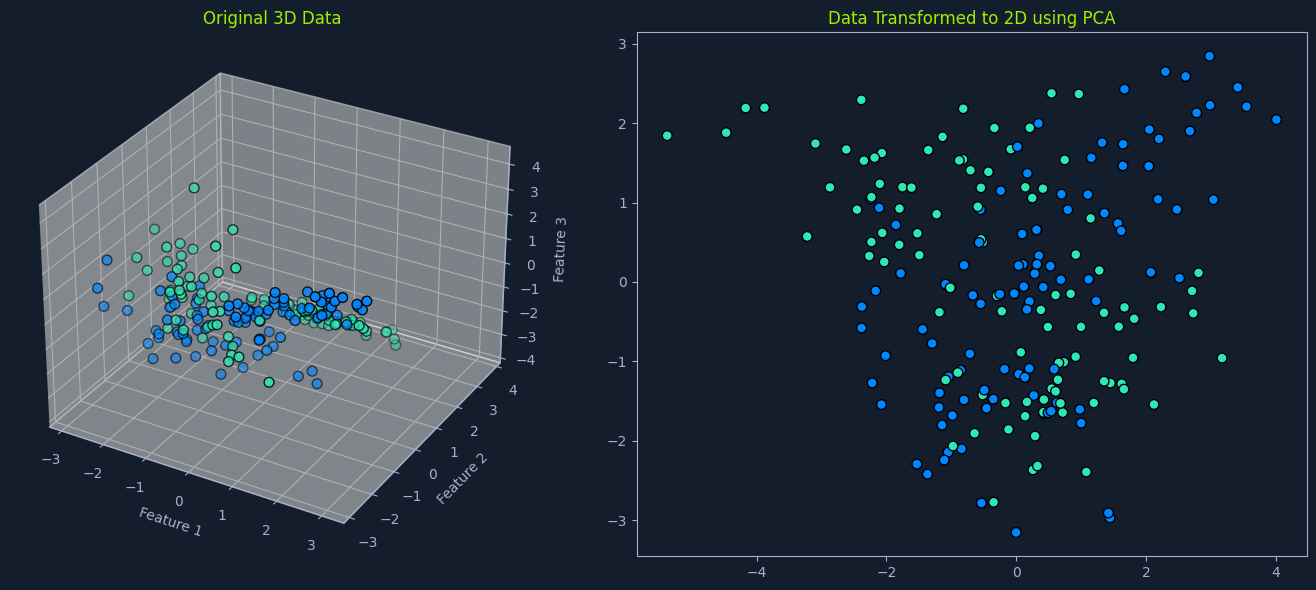
Principal Component Analysis (PCA) is a dimensionality reduction technique that transforms high-dimensional data into a lower-dimensional representation while preserving as much original information as possible. It achieves this by identifying the principal components and new variables that are linear combinations of the original features and capturing the maximum variance in the data. PCA is widely used for feature extraction, data visualization, and noise reduction.
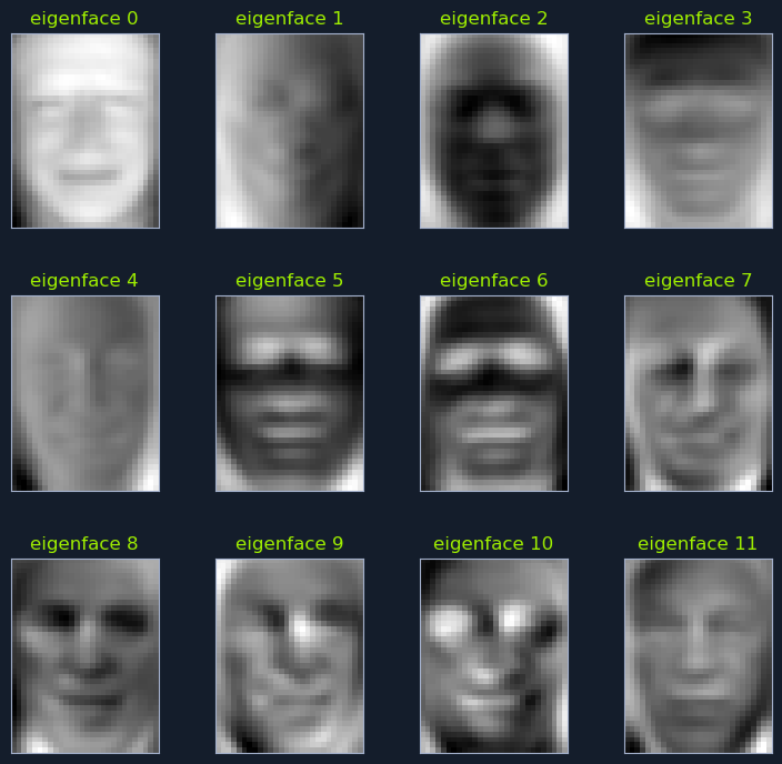
For example, in image processing, PCA can reduce the dimensionality of image data by identifying the principal components that capture the most important features of the images, such as edges, textures, and shapes.
Think of it as finding the most important "directions" in the data. Imagine a scatter plot of data points. PCA finds the lines that best capture the spread of the data. These lines represent the principal components.
Consider a database of facial images. PCA can be used to identify the principal components that capture the most significant variations in facial features, such as eye shape, nose size, and mouth width. By projecting the facial images onto a lower-dimensional space defined by these principal components, we can efficiently search for similar faces.
There are three key concepts to PCA:
- Variance: - Variance measures the spread or dispersion of data points around the mean. PCA aims to find principal components that maximize variance, capturing the most significant information in the data.
- Covariance: - Covariance measures the relationship between two variables. PCA considers the covariance between different features to identify the directions of maximum variance.
- Eigenvectors and Eigenvalues: - Eigenvectors represent the directions of the principal components, and eigenvalues represent the amount of variance explained by each principal component.
The PCA algorithm follows these steps:
- Standardize the data: - Subtract the mean and divide by the standard deviation for each feature to ensure that all features have the same scale.
- Calculate the covariance matrix: - Compute the covariance matrix of the standardized data, which represents the relationships between different features.
- Compute the eigenvectors and eigenvalues: - Determine the eigenvectors and eigenvalues of the covariance matrix. The eigenvectors represent the directions of the principal components, and the eigenvalues represent the amount of variance explained by each principal component.
- Sort the eigenvectors: - Sort the eigenvectors in descending order of their corresponding eigenvalues. The eigenvectors with the highest eigenvalues capture the most variance in the data.
- Select the principal components: - Choose the top k eigenvectors, where k is the desired number of dimensions in the reduced representation.
- Transform the data: - Project the original data onto the selected principal components to obtain the lower-dimensional representation.
By following these steps, PCA can effectively reduce the dimensionality of a dataset while retaining the most important information.
Eigenvalues and Eigenvectors
Before diving into the eigenvalue equation, it's important to understand what eigenvectors and eigenvalues are and their significance in linear algebra and machine learning.
An eigenvector is a special vector that remains in the same direction when a linear transformation (such as multiplication by a matrix) is applied to it. Mathematically, if A is a square matrix and v is a non-zero vector, then v is an eigenvector of A if:
A * v = λ * v
Here, λ (lambda) is the eigenvalue associated with the eigenvector v.
The eigenvalue λ represents the scalar factor by which the eigenvector v is scaled during the linear transformation. In other words, when you multiply the matrix A by its eigenvector v, the result is a vector that points in the same direction as v but stretches or shrinks by a factor of λ.
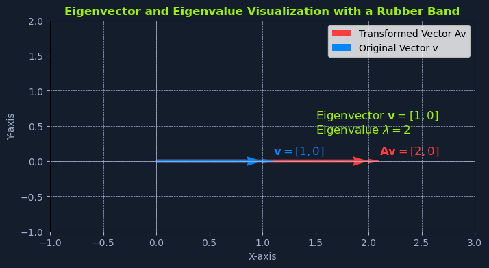
Consider a rubber band stretched along a coordinate system. A vector can represent the rubber band, and we can transform it using a matrix.
Let's say the rubber band is initially aligned with the x-axis and has a length of 1 unit. This can be represented by the vector v = [1, 0].
Now, imagine applying a linear transformation (stretching it) represented by the matrix A:
          A = [[2, 0],
              [0, 1]]
When we multiply the matrix A by the vector v, we get:
          A * v = [[2, 0],
                  [0, 1]] * [1, 0] = [2, 0]
The resulting vector is [2, 0], which points in the same direction as the original vector v but has been stretched by a factor of 2. The eigenvector is v = [1, 0], and the corresponding eigenvalue is λ = 2.
The Eigenvalue Equation in Principal Component Analysis (PCA)
In Principal Component Analysis (PCA), the eigenvalue equation helps identify the principal components of the data. The principal components are obtained by solving the following eigenvalue equation:
          C * v = λ * v

          Where:
            C is the standardized data's covariance matrix. This matrix represents the relationships between different features, with each element indicating the covariance between two features.
            v is the eigenvector. Eigenvectors represent the directions of the principal components in the feature space, indicating the directions of maximum variance in the data.
            λ is the eigenvalue. Eigenvalues represent the amount of variance explained by each corresponding eigenvector (principal component). Larger eigenvalues correspond to eigenvectors that capture more variance.
Solving the Eigenvalue Equation
Solving this equation involves finding the eigenvectors and eigenvalues of the covariance matrix. This can be done using techniques like:
- Eigenvalue Decomposition: - Directly computing the eigenvalues and eigenvectors.
- Singular Value Decomposition (SVD): - A more numerically stable method that decomposes the data matrix into singular vectors and singular values related to the eigenvectors and eigenvalues of the covariance matrix.
Selecting Principal Components
Once the eigenvectors and eigenvalues are found, they are sorted in descending order of their corresponding eigenvalues. The top k eigenvectors (those with the largest eigenvalues) are selected to form the new feature space. These top k eigenvectors represent the principal components that capture the most significant variance in the data.
The transformation of the original data X into the lower-dimensional representation Y can be expressed as:
          Y = X * V

          Where:
            Y is the transformed data matrix in the lower-dimensional space.
            X is the original data matrix.
            V is the matrix of selected eigenvectors.
This transformation projects the original data points onto the new feature space defined by the principal components, resulting in a lower-dimensional representation that captures the most significant variance in the data. This reduced representation can be used for various purposes such as visualization, noise reduction, and improving the performance of machine learning models.
Choosing the Number of Components
The number of principal components to retain is a crucial decision in PCA. It determines the trade-off between dimensionality reduction and information preservation.
A common approach is to plot the explained variance ratio against the number of components. The explained variance ratio indicates the proportion of total variance captured by each principal component. By examining the plot, you can choose the number of components that capture a sufficiently high percentage of the total variance (e.g., 95%). This ensures that the reduced representation retains most of the essential information from the original data.
Data Assumptions
PCA makes certain assumptions about the data:
- Linearity: - It assumes that the relationships between features are linear.
- Correlation: - It works best when there is a significant correlation between features.
- Scale: - It is sensitive to the scale of the features, so it is important to standardize the data before applying PCA.
PCA is a powerful technique for dimensionality reduction and data analysis. It can simplify complex datasets, extract meaningful features, and visualize data in a lower-dimensional space. However, knowing its assumptions and limitations is important to ensure its effective and appropriate application.